New Zealanders are warned of scam text messages currently circulating that claim to be from the Ministry of Justice about overdue traffic fines. The Ministry does not include any links in our texts. Read more about Texts from Ministry of Justice
The three types of statistics used in NZCASS reporting are:
Percentages – for example 24% of adults were a victim of crime once or more in 2013.
Averages – for example on average 69 offences were experienced for every 100 adults in 2013 (incidence rates). Incidence rates are a type of average, and averages are also used for the incident mean seriousness score.
Totals – for example the estimated total number of burglary offences in 2013 was 203,000. Totals are mainly used in crime rate tables.
These statistics are always weighted and in the data tables given with their sampling error. While we used standard methods to analyse these statistics, NZCASS has some complexities that we explain on this page:
the use of replicate weights to estimate sampling error
the use of imputed data
the tests used to assess statistical significance.
We used a replicate weight technique to estimate sampling error for NZCASS. These methods are well established for use in surveys with complex sample designs and weighting procedures.
The method used was the delete-a-group Jackknife method, where 100 replicate weights were calculated to accompany the main weight. See Weighting for how we calculated the main weights. We calculated replicate weights by dividing the main sample into 100 groups, and leaving out one group from the sample at a time to form each replicate. We re-ran the weighting process for each of the 100 replicate groups, to produce 100 replicate weights.
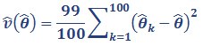
We then used these 100 replicate weights to calculate the sampling error of the estimate. This is done by calculating the statistic of interest for the main weight and for each of the 100 replicate weights. The variance estimate for unimputed data in NZCASS 2014 is then calculated as:
Equation 1
where θ̂ is the statistic of interest calculated using the main survey weights, and θ̂k is the same statistic calculated using the kth set of replicate weights.
The standard error of the estimate is the square root of this variance estimate. This standard error is then used in the calculation of the relative standard error, the margin of error and confidence intervals. See How variable are results for the definitions of these measures. For confidence intervals of unimputed data, the t-value has 99 degrees of freedom.
We give the sampling error for all NZCASS statistics in the NZCASS data tables.
Imputation is a statistical method to account for missing data. The imputation process assigns 100 imputations for each respondent, which means that the analysis of imputed data is more complex than the standard formula. We calculated estimates and variance estimates for each of the 100 multiple imputation datasets. These statistics were then combined across the 100 imputations using Rubin’s (1987) combining rules as follows:
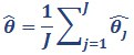
The overall estimate is the average of estimates from each individual imputed dataset:
Equation 2
where J is the number of imputations (100), and θ̂j is the estimate of the statistic for the jth imputed dataset.
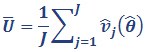
We calculate the variance estimate for statistics involving imputed data from both the within-imputation variance and the between-imputation variance.
Within-imputation variance:
Equation 3
v̂j(θ̂) is the variance estimate for the jth imputed dataset, calculated using replicate weights, as specified in Equation 1.
Between-imputation variance:
Equation 4
where θ̂j is the estimate of the statistic for the jth imputed dataset, and var[θ̂j] is the variance of the statistic’s estimate across the J imputed datasets.
This is combined to yield the total variance estimate:
Equation 5
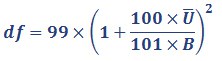
As we explained in How sampling error was calculated, the standard error is the square root of this variance estimate. Confidence intervals are calculated as the estimate (θ̂) plus and minus the standard error multiplied by the t-value. For imputed data, the t-value has the following degrees of freedom for 100 imputations:
How tests of statistical significance were conducted
When estimates are compared over time or between sub-groups within a survey year, the differences between the estimates are tested for statistical significance. We do this to determine if the difference is ‘real’ or simply caused by the survey’s sampling error. We used different significance tests for tests over time and for tests between categories within a survey year. Statistical significance was tested at the 95% confidence level (unless otherwise stated).
Comparisons over time (between surveys)
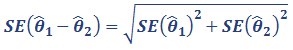
Let θ̂1 = estimate for time 1 (eg 2009)
θ̂2 = estimate for time 2 (eg 2014)
The difference is (y) = θ̂1 – θ̂2. The standard error of the difference is approximated by:
Equation 7
If the confidence interval for this difference contains 0, then the difference is considered not statistically significant.
Comparisons between sub-groups within one survey
We used different tests of significance for different statistics:
t-tests were used to determine statistical differences in averages (incidence rates and means) and totals
rate ratios were used to determine statistical differences in percentages (including prevalence rates).
t-test
Let θ̂A = estimate for Group A
θ̂B = estimate for Group B
The difference is (y) = θ̂A – θ̂B. The variance of the difference is calculated using Equation 1 where θ ̂ in this equation is the difference (y). Likewise, variance estimates for data involving imputation are given by Equation 5.
If the confidence interval contains 0, then the difference is not considered statistically significant.
Rate ratio test
Let P̂A = percentage for Group A
P̂B = percentage for Group B
The rate ratio r̂A,B = P̂A/P̂B. The variance of the rate ratio is calculated in a log scale using Equation 1 where θ̂ in this equation is the log of the rate ratio, ie ln(r̂A,B). Variance estimates for rate ratios for data involving imputation are given by Equation 5. The confidence interval is formed by taking the exponential of the lower and upper bounds calculated from the log of the rate ratio.
If the confidence interval contains 1, then the difference is not considered statistically significant.
What modelling was done and where you can find more information
We used different types of analysis to help us better understand different aspects of crime and victimisation. The three advanced statistical methods of modelling used as part of NZCASS were:
Multiple standardisation – a reweighting technique to address the question: if the demographic profile between Māori and Europeans was the same as the combined average, would Māori still be more highly victimised?
Logistic regression – a common multivariate analysis technique that we used to identify the strongest predictors of victimisation for difference offence types.
The Gini coefficient – summarises the distribution of victimisation in a single statistic and allows us to make comparisons over time and between groups.
Download advanced statistical methods for detail on the modelling aims, methods and results for these three methods.